2 Activities: Introductory
2.1 Getting Started in RStudio
2.1.1 Review + Assignment
As you might guess from the name, “Data Science” requires data. Working with modern (large, messy) data sets requires statistical software. We’ll exclusively use RStudio. Why?
- it’s free
- it’s open source (the code is free & anybody can contribute to it)
- it has a huge online community (which is helpful for when you get stuck)
- it’s one of the industry standards
- it can be used to create reproducible and lovely documents (In fact, this entire course manual that you’re currently reading was constructed entirely within RStudio!)
Download R & RStudio
To get started, take the following two steps in the given order. Even if you already have R/RStudio, make sure to update to the most recent versions. Further, if you get stuck, visit the ITS help desk.
STEP 1: Download & install the R statistical software at https://mirror.las.iastate.edu/CRAN/
STEP 2: Download & install the FREE version of RStudio at https://www.rstudio.com/products/rstudio/download/
What’s the difference between R and RStudio? Mainly, RStudio requires R – thus it does everything R does and more. We will be using RStudio exclusively.
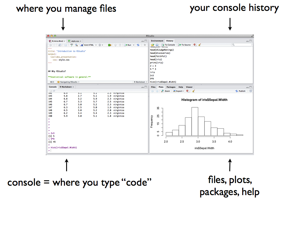
Open RStudio! You should see four panes, each serving a different purpose:

- Warm-Up
- Perform a simple calculation: calculate
90/3.
- RStudio has built-in functions to which we supply the necessary arguments:
function(arguments). Use a built-in function to calculate the square root of 25.
- Use a built-in function to repeat the number “5” 8 times.
- Use the
seqfunction to create the vector(0, 3, 6, 9, 12). (The video doesn’t cover this!)
- Repeat this vector 3 times.
- Perform a simple calculation: calculate
- Assignment
We often want to store our output for later use (why?). The basic idea in RStudio:
name <- outputTry the following syntax line by line. NOTE: RStudio ignores any content after the
#. Thus we use this to ‘comment’ and organize our code.#type square_3 square_3 #calculate 3 squared 3^2 #store this as "square_3" square_3 <- 3^2 #type square_3 again! square_3 #do some math with square_3 square_3 + 2
2.1.2 Tidy Data
Not only does “Data Science” require statistical software, it requires DATA! Consider the Google definition:
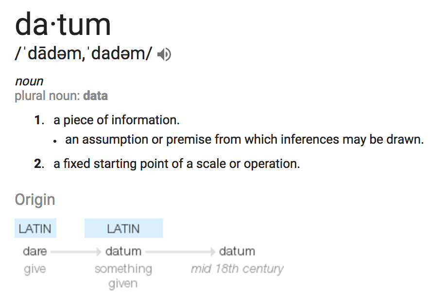
Types of Data
With this definition in mind, which of the following are examples of data?
tables
##   family father mother sex height nkids
## 1      1   78.5   67.0   M   73.2     4
## 2      1   78.5   67.0   F   69.2     4
## 3      1   78.5   67.0   F   69.0     4
## 4      1   78.5   67.0   F   69.0     4
## 5      2   75.5   66.5   M   73.5     4
## 6      2   75.5   66.5   M   72.5     4
Converting to Data Tables
We’ll mostly work with data that look like this:
##   family father mother sex height nkids
## 1      1   78.5   67.0   M   73.2     4
## 2      1   78.5   67.0   F   69.2     4
## 3      1   78.5   67.0   F   69.0     4
## 4      1   78.5   67.0   F   69.0     4
## 5      2   75.5   66.5   M   73.5     4
## 6      2   75.5   66.5   M   72.5     4
This isn’t as restrictive as it seems. How can we convert the above signals, photos, videos, and text to a data table format?
Example
After a scandal among FIFA officials, fivethirtyeight.com posted an analysis of FIFA viewership, How to Break FIFA. Here’s a snapshot of the data used in this article:
| country | confederation | population_share | tv_audience_share | gdp_weighted_share |
|---|---|---|---|---|
| United States | CONCACAF | 4.5 | 4.3 | 11.3 |
| Japan | AFC | 1.9 | 4.9 | 9.1 |
| China | AFC | 19.5 | 14.8 | 7.3 |
| Germany | UEFA | 1.2 | 2.9 | 6.3 |
| Brazil | CONMEBOL | 2.8 | 7.1 | 5.4 |
| United Kingdom | UEFA | 0.9 | 2.1 | 4.2 |
| Italy | UEFA | 0.9 | 2.1 | 4.0 |
| France | UEFA | 0.9 | 2.0 | 4.0 |
| Russia | UEFA | 2.1 | 3.1 | 3.5 |
| Spain | UEFA | 0.7 | 1.8 | 3.1 |
Tidy Data
The data table above is in tidy format. Tidy data tables have three key features:
- Each row represents a unit of observation.
- Each column represents a variable (ie. an attribute of the cases that can vary from case to case). Each variable is 1 of 2 types:
- quantitative = numerical
- categorical = discrete possibilities/categories
- Contains only data, no analysis, summaries, footnotes, comments, etc.
- Units of observation & Variables
- What are the units of observation in the FIFA data?
- What are the variables? Which are quantitative? Which are categorical?
- Are these tidy data?
- What are the units of observation in the FIFA data?
- Tidy vs Untidy
Check out the following data. Explain why they are untidy and how we can tidy them.Data 1: FIFA
country confederation population share tv_share United States CONCACAF i don’t know* 4.3% *look up later Japan AFC 1.9 4.9% China AFC 19.5 14.8% total=24% Data 2: Gapminder life expectancies by country
country 1952 1957 1962 Asia Afghanistan 28.8 30.3 32.0 Bahrain 50.9 53.8 56.9 Africa Algeria 43.0 45.7 48.3
2.1.3 Data Basics in RStudio
For now, we’ll focus on tidy data. In a couple of weeks, you’ll learn how to turn untidy data into tidy data.
Import data
The first step to working with data in RStudio is getting it in there! How we do this depends on its format (eg: Excel spreadsheet, csv file, txt file) and storage locations (eg: online, within Wiki, desktop). Luckily for us, thefifa_audiencedata are stored in thefivethirtyeightRStudio package.#load the fivethirtyeight package library(fivethirtyeight) #load the fifa data data("fifa_audience") #store this under a shorter, easier name fifa <- fifa_audience
Examining data structure
Before we can analyze our data, we must understand its structure. Try out the following functions. For each, write a comment after#that describes its action.#(what does View do?) View(fifa) #(what does head do?) head(fifa) #(what does dim do?) dim(fifa) #(what does names do?) names(fifa)
Codebooks
Data are also only useful if we know what they measure! Thefifadata table is tidy – it doesn’t have any helpful notes. Rather, information about the data is stored in a separate codebook. Codebooks can be stored in many ways (eg: Google docs, word docs, etc). Here the authors have made their codebook available in RStudio (under the originalfifa_audiencename). Check it out:?fifa_audience- What does
population_sharemeasure?
- What are the units of
population_share?
- What does
- Examining a single variable
We might want to access & focus on a single variable. To this end, we can use the
$notation:fifa$tv_audience_share fifa$confederationIt’s important to understand the format/class of each variable (quantitative, categorical, date, etc) in both its meaning and its structure within RStudio:
class(fifa$tv_audience_share)
class(fifa$confederation)
If a variable is categorical (either in
characterorfactorformat), we can determine itslevels/ category labels:levels(fifa$confederation) levels(factor(fifa$confederation))
- New data!
There’s a data set namedcomic_charactersin thefivethirtyeightpackage.- Load the data.
- Give a 1 sentence summary of what these data measure. (HINT: codebook!)
- What are the units of observation? How many observations are there?
- Examine the first rows of the data set.
- What’s the class of the
datevariable?
- Get a list of all variable names.
- Load the data.
2.2 R Markdown and Reproducible Research
Reproducible research is the idea that data analyses, and more generally, scientific claims, are published with their data and software code so that others may verify the findings and build upon them. - Reproducible Research, Coursera
Useful Resources:
Research often makes claims that are difficult to verify. A recent study of published psychology articles found that less than half of published claims could be reproduced. One of the most common reasons claims cannot be reproduced is confusion about data analysis. It may be unclear exactly how data was prepared and analyzed, or there may be a mistake in the analysis.
In this course we will use an innovative new format called R Markdown that dramatically increases the transparency of data analysis. R Markdown interleaves data, R code, graphs, tables, and text and packages it an easily writeable and publishable format.
To use R Markdown, you will write an R Markdown formatted file in RStudio and then ask RStudio to knit it into an HTML document (or occasionally a PDF or MS Word document). For an example, take a look at this Sample RMarkdown and the HTML webpage it creates.
Deduce the R Markdown Format Look at the Rmd and HTML page side-by-side linked above.
How are bullets, italics, and section headers represented in the R Markdown file?
How does R code appear in the R Markdown file?
In the HTML webpage, do you see the R code, the output of the R code, or both?
Now take a look at the R Markdown Cheatsheet. Look up the R Markdown features from the previous question on the cheatsheet. There’s a great deal more information there.
Complete the following. If you get stuck along the way, refer to the R Markdown Cheatsheet linked above, search the web for answers, or ask for help!
- Create your first R Markdown file
Create a new R Markdown about your favorite food.- Create a new file in RStudio (File -> New File -> R Markdown) called
First Markdown.
- Make sure you can compile (Knit) the Markdown into a webpage.
- Create a brief essay about your favorite food. Make sure to include:
- Two sections
- A picture from the web
- A bullet list
- A numbered list
- Two sections
- Add R code to your R Markdown
- Print the dimensions of the the bechdel dataset (hint: the bechdel name is available in the fivethirtyeight package)
- Create a second chunk that prints the first few rows of the bechdel dataset.
- Print the dimensions of the the bechdel dataset (hint: the bechdel name is available in the fivethirtyeight package)
- Compile the document.
- Create a new file in RStudio (File -> New File -> R Markdown) called