8 Additional Topics
8.1 Introduction to Text Processing in R
Reading:
In this module you will learn to analyze text. Text refers to information composed primarily of words: song lyrics, Tweets, news articles, novels, Wikipedia articles, online forums, and countless other resources. In R and most other programming languages, text is stored in strings. There are a variety of common ways to get strings containing the text want to analyze.
8.1.1 Getting Started with twitteR
Required modules:
library(tidyverse)
library(tidytext)
library(wordcloud)
library(twitteR)
8.1.2 Getting Strings, Technique 1: String Literals
It may be natural to start by declaring an R variable that holds a string. Let’ consider the U.S. Declaration of Independence. Here’s an R variable that contains one of the most memorable sentences in the Declaration of Independence:
us_dec_sentence <- 'We hold these truths to be self-evident, that all men are created equal, that they are endowed by their Creator with certain unalienable Rights, that among these are Life, Liberty and the pursuit of Happiness.'

# Show the number of characters in the sentence.
nchar(us_dec_sentence)
## [1] 209

# Show the sentence itself.
us_dec_sentence
## [1] "We hold these truths to be self-evident, that all men are created equal, that they are endowed by their Creator with certain unalienable Rights, that among these are Life, Liberty and the pursuit of Happiness."
Unfortunately, creating literal string variables like this can become unwieldy for larger texts, or collections of multiple texts. Using this technique, your R program would be narrowly written to analyze hard-coded string variables, and defining those string variables may take up the vast majority of our program’s source code, making it difficult to read. We will discuss two more flexible ways of getting textual data: reading a .TXT file and accessing a web API.
8.1.3 Getting Strings, Technique 2: Reading .txt Files
We will learn to analyze the simplest file format for text: a .TXT file. A .txt file contains raw textual data.
You can find .TXT files by using Google’s filetype: search filter. Go to http://google.com and type filetype:txt declaration of independence in the search box. In the results you should see many .txt files containing the U.S. Declaration of Independence. For example, https://www.usconstitution.net/const.txt.
Open https://www.usconstitution.net/const.txt in your browser and save the file. Run file.choose() to determine the correct path to the file on your computer.
# Run file.choose() to find the right path below on your computer
library(readr)
us_dec <- read_file("./const.txt")
Read the .txt file into R as a string using the readr package. Because the text is so large, we use the strtrim function to only show the first 500 characters of the text.
nchar(us_dec)
## [1] 45119
strtrim(us_dec, 500)
## [1] "Provided by USConstitution.net\n------------------------------\n\n[Note: Repealed text is not noted in this version.  Spelling errors have been\ncorrected in this version.  For an uncorrected, annotated version of the\nConstitution, visit http://www.usconstitution.net/const.html ]\n\nWe the People of the United States, in Order to form a more perfect Union,\nestablish Justice, insure domestic Tranquility, provide for the common\ndefence, promote the general Welfare, and secure the Blessings of Liberty to"
Notice all those \n sequences that appear in the string. These are newline characters that denote the end of a line. There are a few other special characters that you may see. For example, '\t' is a tab.
8.1.4 Analyzing Single Documents
If we tried to make a dataframe directly out of the text it would look odd. It contains the text as a single row in a column named “text”. This doesn’t seem any more useful than the original string itself.
us_dec_df <- data_frame(title = 'Declaration of Independence', text = us_dec)
us_dec_df
## # A tibble: 1 x 2
##                         title
##                         <chr>
## 1 Declaration of Independence
## # ... with 1 more variables: text <chr>
We need to restructure the text into two data components that can be easily analyzed. We will use two units of data. A token is the smallest textual information unit we wish to measure, typically a word. A document is a collection of tokens. For our examples here, a document is the Declaration of Indepence. However, a document could be a tweet, a novel chapter, a Wikipedia article, or anything else that seems interesting. We will often perform textual analyses comparing two or more documents.
We will be using the tidy text format, which has one row for each unit of analysis. Our work will focus on word-level analysis within each document, so each row will contain a document and word. TidyText’s unnest_tokens function takes a dataframe containing one row per document and breaks it into a data frame containing one row per token.
tidy_us_dec <- us_dec_df %>%
  unnest_tokens(word, text)

tidy_us_dec
## # A tibble: 7,663 x 2
##                          title               word
##                          <chr>              <chr>
##  1 Declaration of Independence           provided
##  2 Declaration of Independence                 by
##  3 Declaration of Independence usconstitution.net
##  4 Declaration of Independence               note
##  5 Declaration of Independence           repealed
##  6 Declaration of Independence               text
##  7 Declaration of Independence                 is
##  8 Declaration of Independence                not
##  9 Declaration of Independence              noted
## 10 Declaration of Independence                 in
## # ... with 7,653 more rows
Note that because we only have one document, the initial dataframe is just one row and the tidy text dataframe has the same title for each row. Later on we will analyze more than one document and these columns can change.
We can now analyze this tidy text data frame. For example, we can determine the total number of words.
nrow(tidy_us_dec)
## [1] 7663
We can also find the most frequently used words by using dplyr’s count function, which creates a frequency table for (in our case) words:
# Create and display frequency count table
all_us_dec_counts <- tidy_us_dec %>%
  count(word, sort = TRUE)
all_us_dec_counts
## # A tibble: 1,180 x 2
##         word     n
##        <chr> <int>
##  1       the   727
##  2        of   495
##  3     shall   306
##  4       and   264
##  5        to   202
##  6        be   179
##  7        or   160
##  8        in   147
##  9    states   129
## 10 president   121
## # ... with 1,170 more rows
We can count the rows in this data frame to determine how many different unique words appear in the document.
nrow(all_us_dec_counts)
## [1] 1180
Notice that the most frequent words are common words that are present in any document and not particularly descriptive of the topic of the document. These common words are called stop words, and they are typically removed from textual analysis. TidyText provides a built in set of 1,149 different stopwords. We can load the dataset and use anti_join to remove rows associated with words in the dataset.
# Load stop words dataset and display it
data(stop_words)
stop_words
## # A tibble: 1,149 x 2
##           word lexicon
##          <chr>   <chr>
##  1           a   SMART
##  2         a's   SMART
##  3        able   SMART
##  4       about   SMART
##  5       above   SMART
##  6   according   SMART
##  7 accordingly   SMART
##  8      across   SMART
##  9    actually   SMART
## 10       after   SMART
## # ... with 1,139 more rows

# Create and display frequency count table after removing stop words from the dataset
us_dec_counts <- tidy_us_dec %>%
  anti_join(stop_words) %>%
  count(word, sort=TRUE)
us_dec_counts
## # A tibble: 958 x 2
##               word     n
##              <chr> <int>
##  1       president   121
##  2          united    85
##  3        congress    60
##  4             law    39
##  5          office    37
##  6            vice    36
##  7       amendment    35
##  8          person    34
##  9           house    33
## 10 representatives    29
## # ... with 948 more rows
Finally, we can create a word cloud to create a visualization of the most frequent words in the dataset:
library(wordcloud)

# Show a word cloud with some customized options

wordcloud(us_dec_counts$word,             # column of words
          us_dec_counts$n,                # column of frequencies
          scale=c(2,0.1),                 # range of font sizes of words
          min.freq = 2,                   # minimum word frequency to show
          max.words=200,                  # show the 200 most frequent words
          random.order=FALSE,             # position the most popular words first
          colors=brewer.pal(8, "Dark2"))  # Color palette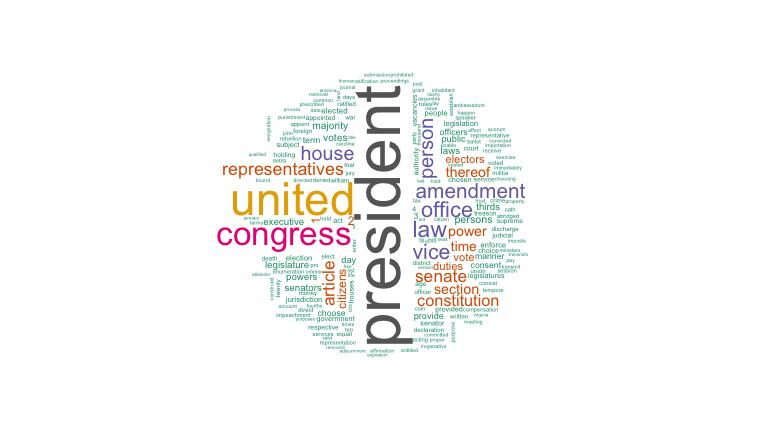
Setting up Twitter Authentication
We will be analyzing the text of tweets about different topics for this assignment. In order to get data from Twitter, we need to setup OAuth authentication between Twitter and R. OAuth is a more sophisticated authentication scheme than the key-based authentication we used for the NY Times, and it is used by social APIs such as Facebook, LinkedIn, and others. We do this by creating a Twitter “app” for our R code:
Login to your Twitter account. If you don’t have a Twitter account, you will need to create one.
Click the “create new app” button.
Name your app “comp-112,” give it some description, enter http://www.macalester.edu for the website, and agree to the developer agreement. Then click the “Create your Twitter application” button.
Click on the “Keys and Access Tokens” tab, and record the “Consumer Key” and “Consumer Secret” in variables in your rmarkdown.
Click “Create my access token” and record the access token and access token secret in variables in your rmarkdown.
Make sure there are not extra spaces around any of the four R variables you created in the last step.
# Replace these with the values for your Twitter Application.
apiKey = "asdfasfasdfas"
apiSecret = "aasdfasdagerqwasdvxcvz"
accessToken = "asfasdfdasf"
accessTokenSecret = "asfasdfdasf"
Next, configure your twitteR account in R. Running the following will pop up a question in the RStudio Console in the bottom left of your Window: Use a local file (‘.httr-oauth’), to cache OAuth access credentials between R sessions? 1: Yes 2: No. Type 1 in the console.
setup_twitter_oauth(apiKey, apiSecret, accessToken, accessTokenSecret)
## [1] "Using direct authentication"
8.1.5 Getting Strings Technique 3: Web APIs
Now we can get tweets on some topic. We are going to use Tweets about “Franken”“, but you can use Tweets about any topic (including a hashtag). The Search API only returns a sample of Tweets created during the last week, so you should pick a topic that is reasonably popular. As with the NYTimes API, asking for a large number of Tweets (in this case 100) results in many API calls, so be careful not to set this number too high or you may face rate limiting.
# Grab up to 200 tweets over the last week that contain the phrase "franken"
frankenTweets <-  searchTwitter('franken', n=200)
frankenTweetsDF <- twListToDF(frankenTweets)
head(frankenTweetsDF)
##                                                                                                                                             text
## 1    @missydiggs @xmssweetnessx But it's still 3% of what total number ? And not to mention you're referring to serious… https://t.co/FLjqfoQudu
## 2        @carrieksada @BreitbartNews @steph93065 @CarmineZozzora @AmericanHotLips @AppSame @SparkleSoup45 @RuthieRedSox… https://t.co/VWX9zy14GL
## 3         RT @Gardianofcross: "Jessica Leeds"\nLook at that face.\nTrump would not touch that woman.\nAl Franken wouldn't even grope that woman.
## 4 RT @StandUpAmerica: Donald Trump's accusers speak out—and call for an investigation.\n\n"I think if [Congress] was willing to investigate Sen…
## 5                                RT @washingtonpost: In Franken’s wake, three senators call on President Trump to resign https://t.co/XOVHWr6H3g
## 6   RT @turnercampdave: @DearAuntCrabby @alfranken https://t.co/SKafKHKJRC. This is how I feel.  I feel it has discredited woman who were reall…
##   favorited favoriteCount   replyToSN             created truncated
## 1     FALSE             0  missydiggs 2017-12-11 17:35:57      TRUE
## 2     FALSE             0 carrieksada 2017-12-11 17:35:56      TRUE
## 3     FALSE             0        <NA> 2017-12-11 17:35:55     FALSE
## 4     FALSE             0        <NA> 2017-12-11 17:35:55     FALSE
## 5     FALSE             0        <NA> 2017-12-11 17:35:52     FALSE
## 6     FALSE             0        <NA> 2017-12-11 17:35:51     FALSE
##           replyToSID                 id replyToUID
## 1 940245272399155200 940273966287147008   38004751
## 2 939969709423726592 940273963288219648 2596413645
## 3               <NA> 940273956807901184       <NA>
## 4               <NA> 940273955184750592       <NA>
## 5               <NA> 940273943289536512       <NA>
## 6               <NA> 940273940592594947       <NA>
##                                                                           statusSource
## 1 <a href="http://twitter.com/download/android" rel="nofollow">Twitter for Android</a>
## 2                   <a href="http://twitter.com" rel="nofollow">Twitter Web Client</a>
## 3    <a href="http://twitter.com/#!/download/ipad" rel="nofollow">Twitter for iPad</a>
## 4 <a href="http://twitter.com/download/android" rel="nofollow">Twitter for Android</a>
## 5   <a href="http://twitter.com/download/iphone" rel="nofollow">Twitter for iPhone</a>
## 6 <a href="http://twitter.com/download/android" rel="nofollow">Twitter for Android</a>
##    screenName retweetCount isRetweet retweeted longitude latitude
## 1     Nardo58            0     FALSE     FALSE        NA       NA
## 2     369LuLu            0     FALSE     FALSE        NA       NA
## 3 MarcelThorn            2      TRUE     FALSE        NA       NA
## 4    lynnfc50           22      TRUE     FALSE        NA       NA
## 5  lucysindhu         3100      TRUE     FALSE        NA       NA
## 6    akeleven           30      TRUE     FALSE        NA       NA
We are going to “stick” together the text of each tweet into a giant string:
frankenText <- paste(frankenTweetsDF$text, sep = " ", collapse = "\n")
nchar(frankenText)
## [1] 26456
strtrim(frankenText, 200)
## [1] "@missydiggs @xmssweetnessx But it's still 3% of what total number ? And not to mention you're referring to serious… https://t.co/FLjqfoQudu\n@carrieksada @BreitbartNews @steph93065 @CarmineZozzora @Ame"
And we will follow the same procedure to generate word cloud:
frankenTextDf <- data_frame(query = c("Franken"), text = c(frankenText))

# Unnest the data frame so each row corresponds to a single word in a single document.
frankenTidyDf <- frankenTextDf %>%
  unnest_tokens(word, text)
frankenTidyDf
## # A tibble: 4,114 x 2
##      query          word
##      <chr>         <chr>
##  1 Franken    missydiggs
##  2 Franken xmssweetnessx
##  3 Franken           but
##  4 Franken          it's
##  5 Franken         still
##  6 Franken             3
##  7 Franken            of
##  8 Franken          what
##  9 Franken         total
## 10 Franken        number
## # ... with 4,104 more rows

franken_counts <- frankenTidyDf %>%
  anti_join(stop_words) %>%
  count(word, sort=TRUE)
franken_counts
## # A tibble: 803 x 2
##           word     n
##          <chr> <int>
##  1     franken   142
##  2          rt   141
##  3       https    77
##  4        t.co    74
##  5          al    63
##  6       trump    49
##  7      resign    40
##  8    senators    26
##  9     senator    25
## 10 resignation    24
## # ... with 793 more rows
wordcloud(franken_counts$word, franken_counts$n,
          max.words=200, random.order=FALSE, colors=brewer.pal(8, "Dark2"))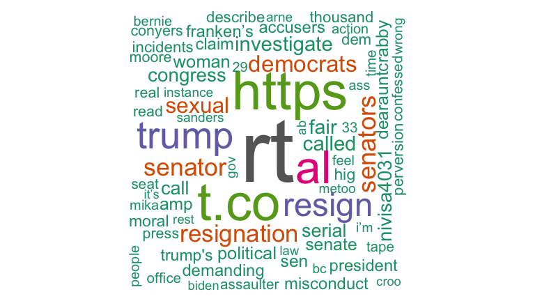
Let’s compare this to tweets about Senator Klobuchar:
klobucharTweets <- searchTwitter('klobuchar', n=200)klobucharTweetsDf <- twListToDF(klobucharTweets)
klobucharText <- paste(klobucharTweetsDf$text, sep = " ", collapse = "\n")
klobucharTextDf <- data_frame(query = c("Klobuchar"), text = c(klobucharText))
klobucharTidyDf <- klobucharTextDf %>%
unnest_tokens(word, text)
klobuchar_counts <- klobucharTidyDf %>%
anti_join(stop_words) %>%
count(word, sort=TRUE)
wordcloud(klobuchar_counts$word, klobuchar_counts$n,
max.words=200, random.order=FALSE, colors=brewer.pal(8, "Dark2"))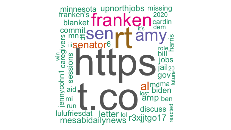
8.1.6 Comparing multiple documents
Let’s compare multiple documents. In particular, we will compare tweets about four senators: Amy Klobuchar and Al Franken (from MN), Lisa Murkowski (AK) and Elizabeth Warren (MA). We need to grab tweets that mention the latter two and form a single text string from them.
Make Twitter API calls:
warrenTweets <-  searchTwitter('warren', n=200)
murkowskiTweets <-  searchTwitter('murkowski', n=200)
Translate them to strings:
warrenTweetsDf <- twListToDF(warrenTweets)
warrenText <- paste(warrenTweetsDf$text, sep = " ", collapse = "\n")
murkowskiTweetsDf <- twListToDF(murkowskiTweets)
murkowskiText <- paste(murkowskiTweetsDf$text, sep = " ", collapse = "\n")
Finally, we construct a single dataframe with all four twitter documents and convert it to tidytext and count the number of words per document:
messySenateDf <- data_frame(
    senator = c("Franken", "Klobuchar", "Warren", "Murkowksi"),
    text = c(frankenText, klobucharText, warrenText, murkowskiText))

tidySenateDf <-
    messySenateDf %>%
    unnest_tokens(word, text)

senateCounts <-
    tidySenateDf %>%
    count(word, senator, sort = TRUE)

head(senateCounts)
## # A tibble: 6 x 3
##      word senator     n
##     <chr>   <chr> <int>
## 1     the  Warren   162
## 2  warren  Warren   151
## 3 franken Franken   142
## 4      rt Franken   141
## 5     the Franken   140
## 6      in  Warren   132
Finally, create Tf-Idf scores. TODO: Describe and motivate this.
senateTfIdf <-
    senateCounts %>%
    bind_tf_idf(word, senator, n) %>%
    arrange(desc(tf_idf))

head(senateTfIdf, 15)
## # A tibble: 15 x 6
##             word   senator     n          tf       idf     tf_idf
##            <chr>     <chr> <int>       <dbl>     <dbl>      <dbl>
##  1     klobuchar Klobuchar   120 0.032017076 1.3862944 0.04438509
##  2     murkowski Murkowksi   116 0.027462121 1.3862944 0.03807058
##  3       collins Murkowksi   108 0.025568182 1.3862944 0.03544503
##  4         chuck    Warren    46 0.011917098 1.3862944 0.01652061
##  5 julianassange    Warren    46 0.011917098 1.3862944 0.01652061
##  6  mcresistance    Warren    46 0.011917098 1.3862944 0.01652061
##  7           amy Klobuchar    43 0.011472785 1.3862944 0.01590466
##  8           202 Murkowksi    44 0.010416667 1.3862944 0.01444057
##  9           224 Murkowksi    44 0.010416667 1.3862944 0.01444057
## 10          cher Murkowksi    37 0.008759470 1.3862944 0.01214320
## 11        voting Murkowksi    35 0.008285985 1.3862944 0.01148681
## 12        warren    Warren   151 0.039119171 0.2876821 0.01125388
## 13   politically Murkowksi    33 0.007812500 1.3862944 0.01083042
## 14    puestoloco Murkowksi    33 0.007812500 1.3862944 0.01083042
## 15          save Murkowksi    33 0.007812500 1.3862944 0.01083042