4 Activities: Wrangling

4.1 Data Wrangling: Introduction

In this activity we will use the following packages. Make sure they are installed on your laptop before we get going.

library(tufte)
library(tidyverse)
library(ggplot2)
library(ggmap)
library(tint)
library(mosaicData)
library(lubridate)

The number of daily births in the US varies over the year and from day to day. What’s surprising to many people is that the variation from one day to the next can be huge: some days have only about 80% as many births as others. Why? In this activity we’ll use basic data wrangling skills to understand some drivers of daily births.

The data table Birthdays in the mosaicData package gives the number of births recorded on each day of the year in each state from 1969 to 1988.¹

Birthdays<-Birthdays%>%select(state,date,year,births)

Table 4.1: A subset of the initial birthday data.
state	date	year	births
AK	1969-01-01	1969	14
AL	1969-01-01	1969	174
AR	1969-01-01	1969	78
AZ	1969-01-01	1969	84
CA	1969-01-01	1969	824
CO	1969-01-01	1969	100

4.1.1 Tidy Data

Additional reading:

There are different ways to store and represent the same data. In order to be consistent and to also take advantage of the vectorized nature of R, the tidyverse packages we’ll use provide a set of three interrelated rules/conventions for a dataset to be tidy:

Each variable must have its own column.
Each observation must have its own row.
Each value must have its own cell.

Figure 4.1: Graphical demonstration of tidy data from the RStudio Data Import Cheat Sheet.

One of the first things we’ll often do when acquiring new data is to “tidy it” into this form. For now, we can already start thinking of a data frame (tibble) as a table whose rows are the individual cases and whose columns are the variables on which we have information for each individual observation. Figure 4.1 from the data import cheat sheet summarizes this principle.

4.1.2 Data Verbs

Additional reading:

Wickham and Grolemund, Data Transformation
Kaplan, Data Computing, Chapters 7 and 9

There are six main data transformation verbs in the dplyr library. Each verb takes an input data frame along with additional arguments specifying the action, and returns a new data frame. We’ll examine them in three pairs.

Verbs that change the variables (columns) but not the cases (rows)

The first two verbs change which variables (columns) are included in the data frame, but preserve the same set of cases (rows).

select() chooses which columns to keep, or put another way, deletes those colummns that are not selected. To specify the columns, we can either list them out, or use functions like starts_with(), ends_with(), or contains() to specify the titles of the variables we wish to keep.
mutate() adds one or more columns to the data frame. Each column is a function of the other columns that is applied on a row by row basis. For example, we can use arithmetic operations like adding two other variables or logical operations like checking if two columns are equal, or equal to a target number.

Exercise 1. Getting Started:
- Add two new variables to the Birthdays data: one that has only the last two digits of the year, and one that states whether there were more than 100 births in the given state on the given date.
- Then form a new table that only has three columns: the state and your two new columns
- What does the following operation return: select(Birthdays,ends_with("te"))?

Verbs that change the cases (rows) but not the variables (columns)

The next two verbs change which cases (rows) are included in the data frame, but preserve the same set of variables (columns).

filter() deletes some of the rows by specifying which rows to keep.
arrange() reorders the rows according to a specified criteria. To sort in reverse order based on the variable x, use arrange(desc(x)).
Exercise 2. Filtering and Arranging: Create a table with only births in Massachusetts in 1979, and sort the days from those with the most births to those with the fewest.

When filtering, we often use logical comparison operators like ==, >, <, >= (greater than or equal to), <= (less than or equal to), and %in%, which compares the value to a list of entries. For example, if we want all births in AK, CA, and MA, we can write

filter(Birthdays, state %in% c("AK","CA","MA"))

The c() here is for concatenate, which is how we form vectors in R.

Grouped summaries

summarise() (or equivalently summarize()) takes an entire data frame as input and outputs a single row with one or more summary statistics, such as mean, sum, sd, n_distinct(), or n() (which, like tally(), just counts the number of entries).

summarise(Birthdays,total_births=sum(births),
          average_births=mean(births),
          nstates=n_distinct(state),ncases=n())
##   total_births average_births nstates ncases
## 1     70486538       189.0409      51 372864

So summarise changes both the cases and the variables. Alone, summarise is not all that useful, because we can also access individual variables directly with the dollar sign. For example, to find the total and average births, we can write

sum(Birthdays$births)
## [1] 70486538
mean(Birthdays$births)
## [1] 189.0409

Rather, we will mostly use it to create grouped summaries, which brings us to the last of the six main data verbs.

group_by() groups the cases of a data frame by a specified set of variables. The size of the stored data frame does not actually change (neither the cases nor the variables change), but then other functions can be applied to the specified groups instead of the entire data set. We’ll often use group_by in conjunction with summarise to get a grouped summary.
Exercise 3. Grouping:
1. Find the average number of daily births in each year.
2. Find the average number of daily births in each year, by state.

4.1.3 Piping

Additional reading: * Wickham and Grolemund, Combining Multiple Operations with the Pipe * Wickham and Grolemund, Pipes

Pipes offer an efficient way to execute multiple operations at once. Here is a more efficient way to redo Example ?? with the pipe:

QuickMABirths1979<-
  Birthdays %>%
  filter(state=="MA",year==1979) %>%
  arrange(desc(births))

With the pipe notation, x%>%f(y) becomes f(x,y), where in the first line here, x is Birthdays, the function f is filter, and y is state=="MA",year==1979. The really nice thing about piping is that you can chain together a bunch of different operations without having to save the intermediate results. This is what we have done above by chaining together a filter followed by an arrange.

4.1.4 Manipulating Dates

Additional reading:

Wickham and Grolemund, Date and Times with lubridate

The date variable in Birthdays prints out in the conventional, human-readable way. But it is actually in a format (called POSIX date format) that automatically respects the order of time. The lubridate package contains helpful functions that will extract various information about any date. Here are some you might find useful:

year()
month()
week()
yday() — gives the day of the year as a number 1-366. This is often called the “Julian day.”
mday() — gives the day of the month as a number 1-31
wday() — gives the weekday (e.g. Monday, Tuesday, …). Use the optional argument label=TRUE to have the weekday spelled out rather than given as a number 1-7.

Using these lubridate functions, you can easily look at the data in more detail. For example, we can add columns to the date table for month and day of the week:

Birthdays<-
  Birthdays %>%
  mutate(month=month(date,label=TRUE),
         weekday=wday(date,label=TRUE))

Here is what the data table looks like with our new columns:²

Table 4.2: A subset of the birthday data with additional variables.
state	date	year	births	month	weekday
AK	1969-01-01	1969	14	Jan	Wed
AL	1969-01-01	1969	174	Jan	Wed
AR	1969-01-01	1969	78	Jan	Wed
AZ	1969-01-01	1969	84	Jan	Wed
CA	1969-01-01	1969	824	Jan	Wed
CO	1969-01-01	1969	100	Jan	Wed

4.1.5 Practice

Exercise 4. Piping practice: Make a table showing the five states with the most births between September 9, 1979 and September 11, 1979, inclusive. Arrange the table in descending order of births.
Exercise 5. Seasonality: For this activity, we need to work with data aggregated across the states.
- Create a new data table, DailyBirths, that adds up all the births for each day across all the states. Plot out daily births vs date.
- To examine seasonality in birth rates, look at the number of births aggregated over all the years by
  1. each week
  2. each month
  3. each Julian day
- When are the most babies born? The fewest?

Exercise 6. Day of the Week: To examine patterns within the week, make a box plot showing the number of births by day of the week. Interpret your results.
Exercise 7. Holidays:
Pick a two-year span of the Birthdays that falls in the 1980s, say, 1980/1981. Extract out the data just in this interval, calling it MyTwoYears. (Hint: filter(), year()). Plot out the births in this two-year span day by day. Color each date according to its day of the week. Explain the pattern that you see.

The plot you generate for Exercise ?? should be generally consistent with the weekend effect and seasonal patterns we have already seen; however, a few days each year stand out as excepetions. We are going to examine the hypothesis that these are holidays. You can find a data set listing US federal holidays at http://tiny.cc/dcf/US-Holidays.csv. Read it in as follows:³
```
Holidays <- read.csv("https://tiny.cc/dcf/US-Holidays.csv") %>%
  mutate(date = as.POSIXct(lubridate::dmy(date)))
```
Now let’s update the plot from Exercise ?? to include the holidays.⁴
1. Add a variable to MyTwoYears called is_holiday. It should be TRUE when the day is a holiday, and FALSE otherwise. One way to do this is with the transformation verb %in%, for instance, is_holiday = date %in% Holidays$date. If you have trouble using %in% try Googling for examples.
2. Add a geom_point layer to your plot that sets the color of the points based on the day of the week and the shape of the points based on whether or not the day is a holiday.
3. Finally, some holidays seem to have more of an effect than others. It would be helpful to label them. Use geom_text with the holiday data to add labels to each of the holidays.

Exercise 8. Geography:

In any way you choose, explore the effect of geography on birth patterns. For example, do parents in Minnesota have fewer winter babies than in other states? Which states have the largest increases or decreases in their portion of US births over time? Is the weekend effect less strong for states with a higher percentage of their populations living in rural areas? Pick any issue (not all of these) that interests you, explore it, and create a graphic to illustrate your findings.
Exercise 9. Superstition:

This article from FiveThirtyEight demonstrates that fewer babies are born on the 13th of each month, and the effect is even stronger when the 13th falls on a Friday. If you have extra time or want some extra practice, you can try to recreate the first graphic in the article.

4.1.6 Drills

We are going to practice the six data verbs on the BabyNames dataset:

library(tidyverse)
library(ggplot2)
library(babynames)

head(babynames)
## # A tibble: 6 x 5
##    year   sex      name     n       prop
##   <dbl> <chr>     <chr> <int>      <dbl>
## 1  1880     F      Mary  7065 0.07238433
## 2  1880     F      Anna  2604 0.02667923
## 3  1880     F      Emma  2003 0.02052170
## 4  1880     F Elizabeth  1939 0.01986599
## 5  1880     F    Minnie  1746 0.01788861
## 6  1880     F  Margaret  1578 0.01616737

Create a new version of BabyNames with only year, name, sex, and a boolean (true or false) indicating whether there were more than 2000 babies with that name.
Find the number of total babies per year, sorted by most babies to least babies.
Find the most popular names overall ordered by popularity.
Find the most popular male names overall ordered by popularity.
Find the most popular male names overall ordered by popularity.
Calculate the number of babies born each decade. Calculating the decade may be the trickiest part of this question!
Calculate the most popular female name for each year This is tricky, but try Googling for hints.

Answers:

Create a new version of BabyNames with only year, name, sex, and a boolean (true or false) indicating whether there were more than 2000 babies with that name.

babynames %>%
    mutate(has2000=n > 2000) %>%
    select(year, name, sex, has2000) %>%
    head()
## # A tibble: 6 x 4
##    year      name   sex has2000
##   <dbl>     <chr> <chr>   <lgl>
## 1  1880      Mary     F    TRUE
## 2  1880      Anna     F    TRUE
## 3  1880      Emma     F    TRUE
## 4  1880 Elizabeth     F   FALSE
## 5  1880    Minnie     F   FALSE
## 6  1880  Margaret     F   FALSE

Calculate the number of total babies per year, sorted by most babies to least babies.

babynames %>%
    group_by(year) %>%
    summarize(n=sum(n)) %>%
    arrange(desc(n)) %>%
    head()
## # A tibble: 6 x 2
##    year       n
##   <dbl>   <int>
## 1  1957 4200146
## 2  1959 4156617
## 3  1960 4154877
## 4  1961 4140040
## 5  1958 4131784
## 6  1956 4121274

Calculate the most popular names overall ordered by popularity.


babynames %>%
    group_by(name) %>%
    summarize(n=sum(n)) %>%
    arrange(desc(n)) %>%
    head()
## # A tibble: 6 x 2
##      name       n
##     <chr>   <int>
## 1   James 5144205
## 2    John 5117331
## 3  Robert 4823167
## 4 Michael 4345569
## 5    Mary 4133216
## 6 William 4087556

Calculate the most popular male names overall ordered by popularity.


babynames %>%
    filter(sex=='M') %>%
    group_by(name) %>%
    summarize(n=sum(n)) %>%
    arrange(desc(n)) %>%
    head()
## # A tibble: 6 x 2
##      name       n
##     <chr>   <int>
## 1   James 5120990
## 2    John 5095674
## 3  Robert 4803068
## 4 Michael 4323928
## 5 William 4071645
## 6   David 3589754

Calculate the most popular male names overall ordered by popularity.


babynames %>%
    filter(sex=='F') %>%
    group_by(name) %>%
    summarize(n=sum(n)) %>%
    arrange(desc(n)) %>%
    head()
## # A tibble: 6 x 2
##        name       n
##       <chr>   <int>
## 1      Mary 4118058
## 2 Elizabeth 1610948
## 3  Patricia 1570954
## 4  Jennifer 1464067
## 5     Linda 1451331
## 6   Barbara 1433339

Calculate the number of babies born each decade. Calculating the decade may be the trickiest part of this question!


babynames %>%
    mutate(decade=floor(year/10)*10) %>%
    group_by(decade) %>%
    summarize(n=sum(n)) %>%
    arrange(decade) %>%
    head()
## # A tibble: 6 x 2
##   decade        n
##    <dbl>    <int>
## 1   1880  2408111
## 2   1890  3362531
## 3   1900  4285249
## 4   1910 14831612
## 5   1920 22971499
## 6   1930 21225401

Calculate the most popular female name for each year This is tricky, but try Googling for an answer.


# Shilad Googled "find max in group_by r" and found this:
# https://stackoverflow.com/questions/24237399/how-to-select-the-rows-with-maximum-values-in-each-group-with-dplyr

babynames %>%
    group_by(year) %>%
    filter(n == max(n)) %>%
    arrange(year)
## # A tibble: 136 x 5
## # Groups:   year [136]
##     year   sex  name     n       prop
##    <dbl> <chr> <chr> <int>      <dbl>
##  1  1880     M  John  9655 0.08154630
##  2  1881     M  John  8769 0.08098299
##  3  1882     M  John  9557 0.07831617
##  4  1883     M  John  8894 0.07907324
##  5  1884     M  John  9388 0.07648751
##  6  1885     F  Mary  9128 0.06430479
##  7  1886     F  Mary  9889 0.06432456
##  8  1887     F  Mary  9888 0.06362034
##  9  1888     F  Mary 11754 0.06204374
## 10  1889     F  Mary 11648 0.06155830
## # ... with 126 more rows

4.2 Data Wrangling: Spread, Gather, Wide and Narrow

In this activity we will the following packages:

library(tufte)
library(tidyverse)
library(ggplot2)
library(ggmap)
library(tint)
library(fivethirtyeight)
library(babynames)

Additional reading: * Wickham and Grolemund on spreading and gathering * Chapter 11 of Data Computing by Kaplan

As we are transforming data, it is important to keep in mind what constitutes each case (row) of the data. For example, in the initial BabyName data below, each case is a single name-sex-year combination. So if we have the same name and sex but a different year, that would be a different case.

Table 4.3: Each case is one name-sex-year combination.
year	sex	name	n	prop
1880	F	Mary	7065	0.0723843
1880	F	Anna	2604	0.0266792
1880	F	Emma	2003	0.0205217
1880	F	Elizabeth	1939	0.0198660
1880	F	Minnie	1746	0.0178886
1880	F	Margaret	1578	0.0161674

It is often necessary to rearrange your data in order to create visualizations, run statistical analysis, etc. We have already seen some ways to rearrange the data to change the case. For example, what is the case after performing the following command?

BabyNamesTotal<-babynames %>%
  group_by(name,sex) %>%
  summarise(total=sum(n))

Each case now represents one name-sex combination:

Table 4.4: Narrow format where each case is one name-sex combination.
name	sex	total
Aaban	M	87
Aabha	F	28
Aabid	M	5
Aabriella	F	15
Aada	F	5
Aadam	M	218

In this activity, we are going to learn two new operations to reshape and reorganize the data: spread() and gather().

4.2.1 Spread

We want to find the common names that are the most gender neutral (used roughly equally for males and females). How should we rearrange the data? Well, one nice way would be to have a single row for each name, and then have separate variables for the number of times that name is used for males and females. Using these two columns, we can then compute a third column that gives the ratio between these two columns. That is, we’d like to transform the data into a wide format with each of the possible values of the sex variable becoming its own column. The operation we need to perform this transformation is spread(). It takes a value (total in this case) representing the variable to be divided into multiple new variables, and a key (the original variable sex in this case) that identifies the variable in the initial narrow format data whose values should become the names of the new variables in the wide format data. The entry fill=0 specifies that if there are, e.g., no females named Aadam, we should include a zero in the corresponding entry of the wide format table.

BabyWide<-BabyNamesTotal %>%
  spread(key=sex,value=total,fill=0)

Table 4.5: A wide format with one case per name enables us to examine gender balance.
name	F	M
Aaban	0	87
Aabha	28	0
Aabid	0	5
Aabriella	15	0
Aada	5	0
Aadam	0	218

Now we can choose common names with frequency greater than 25,000 for both males and females, and sort by the ratio to identify gender-neutral names.

Neutral<-BabyWide %>%
  filter(M>25000,F>25000) %>%
  mutate(ratio = pmin(M/F,F/M)) %>%
  arrange(desc(ratio))

Table 4.6: The most gender-neutral common names, in wide format.
name	F	M	ratio
Kerry	48476	49482	0.9796694
Riley	87347	89585	0.9750181
Jackie	90427	78245	0.8652836
Frankie	32626	40105	0.8135145
Jaime	49552	66314	0.7472329
Peyton	62481	45428	0.7270690
Casey	75402	109122	0.6909881
Pat	40124	26732	0.6662347
Jessie	166088	109560	0.6596503
Kendall	54919	33334	0.6069666
Jody	55655	31109	0.5589615
Avery	100768	49216	0.4884090

4.2.2 Gather

Next, let’s filter these names to keep only those with a ratio of 0.5 or greater (no more than 2 to 1), and then switch back to narrow format. We can do this with the following gather() operation. It gathers the columns listed (F,M) at the end into a single column whose name is given by the key (sex), and includes the values in a column called total.

NeutralNarrow<-Neutral %>%
  filter(ratio>=.5) %>%
  gather(key=sex,value=total,F,M)%>%
  select(name,sex,total)%>%
  arrange(name)

Table 4.7: Narrow format for the most gender-neutral common names.
name	sex	total
Casey	F	75402
Casey	M	109122
Frankie	F	32626
Frankie	M	40105
Jackie	F	90427
Jackie	M	78245

4.2.3 Summary Graphic

Here is a nice summary graphic of gather and spread from the RStudio cheat sheet on data import:

4.2.4 The Daily Show Guests

The data associated with this article is available in the fivethirtyeight package, and is loaded into Daily below. It includes a list of every guest to ever appear on Jon Stewart’s The Daily Show.⁵

Daily<-daily_show_guests

year	google_knowledge_occupation	show	group	raw_guest_list
1999	singer	1999-07-26	Musician	Donny Osmond
1999	actress	1999-07-27	Acting	Wendie Malick
1999	vocalist	1999-07-28	Musician	Vince Neil
1999	film actress	1999-07-29	Acting	Janeane Garofalo
1999	comedian	1999-08-10	Comedy	Dom Irrera
1999	actor	1999-08-11	Acting	Pierce Brosnan
1999	director	1999-08-12	Media	Eduardo Sanchez and Daniel Myrick
1999	film director	1999-08-12	Media	Eduardo Sanchez and Daniel Myrick
1999	american television personality	1999-08-16	Media	Carson Daly
1999	actress	1999-08-17	Acting	Molly Ringwald
1999	actress	1999-08-18	Acting	Sarah Jessica Parker

Exercise 1. Popular Guests:

Create the following table containing 19 columns. The first column should have the ten guests with the highest number of total apperances on the show, listed in descending order of number of appearances. The next 17 columns should show the number of appearances of the corresponding guest in each year from 1999 to 2015 (one per column). The final column should show the total number of appearances for the corresponding guest over the entire duration of the show (these entries should be in decreasing order).⁶

4.2.5 Recreating a Graphic

The original data has 18 different entries for the group variable:

unique(Daily$group)
##  [1] "Acting"         "Comedy"         "Musician"       "Media"         
##  [5] NA               "Politician"     "Athletics"      "Business"      
##  [9] "Advocacy"       "Political Aide" "Misc"           "Academic"      
## [13] "Government"     "media"          "Clergy"         "Science"       
## [17] "Consultant"     "Military"

In order to help you recreate the first figure from the article, I have added a new variable with three broader groups: (i) entertainment; (ii) politics, business, and government, and (iii) commentators. We will learn in the next activity what the inner_join in this code chunk is doing.

DailyGroups<-read_csv("https://www.macalester.edu/~dshuman1/data/112/daily-group-assignment.csv")
Daily<-Daily%>%
  inner_join(DailyGroups,by=c("group"="group"))

year	google_knowledge_occupation	show	group	raw_guest_list	broad_group
1999	actor	1999-01-11	Acting	Michael J. Fox	Entertainment
1999	comedian	1999-01-12	Comedy	Sandra Bernhard	Entertainment
1999	television actress	1999-01-13	Acting	Tracey Ullman	Entertainment
1999	film actress	1999-01-14	Acting	Gillian Anderson	Entertainment
1999	actor	1999-01-18	Acting	David Alan Grier	Entertainment
1999	actor	1999-01-19	Acting	William Baldwin	Entertainment

Exercise 2. Recreating the Graphic:

Using the group assignments contained in the broad_group variable, recreate the graphic from the article, with three different lines showing the fraction of guests in each group over time. Hint: first think about what your case should be for the glyph-ready form.

4.2.6 Gathering Practice

A typical situation that requires a gather command is when the columns represent the possible values of a variable. Table 4.8 shows example data set from opendataforafrica.org with different years in different columns.

Lesotho<-read_csv("https://www.macalester.edu/~dshuman1/data/112/Lesotho.csv")

Table 4.8: Financial statistics about Lesotho.
Category	2010	2011	2012	2013	2014
Total Population	2.01	2.03	2.05	2.07	2.10
Gross Domestic Product	2242.30	2560.99	2494.60	2267.96	1929.28
Average Interest Rate on Loans	11.22	10.43	10.12	9.92	10.34
Inflation Rate	3.60	4.98	6.10	5.03	4.94
Average Interest Rate on Deposits	3.68	2.69	2.85	2.85	2.73

Exercise 3. Gathering practice:

Make a side-by-side bar chart with the year on the horizontal axis, and three side-by-side vertical columns for average interest rate on deposits, average interest rate on loans, and inflation rate for each year. In order to get the data into glyph-ready form, you’ll need to use gather.⁷

4.2.7 Practice Solutions:

Exercise 1: Popular Guests

We can first group by year and guest, then summarise to find the appearances of each guest for each year, then spread into a wider format, then add a column with total appearances over all years, and finally sort in descending order.

PopularDailyWide<-Daily %>%
  group_by(year, raw_guest_list) %>%
  summarise(appearances=n())%>%
  spread(key=year,value=appearances,fill=0)
PopularDailyWide<-PopularDailyWide %>%
  mutate(total=rowSums(PopularDailyWide[,2:18]))%>%
  arrange(desc(total)) %>%
  head(n=10)

raw_guest_list	1999	2000	2001	2002	2003	2004	2005	2006	2007	2008	2009	2010	2011	2012	2013	2014	2015	total
Fareed Zakaria	0	0	1	0	1	2	2	2	1	2	2	1	1	1	1	1	1	19
Denis Leary	1	0	1	2	1	0	0	1	1	2	1	1	2	2	0	1	1	17
Brian Williams	0	0	0	0	1	1	2	1	1	3	2	2	1	1	1	0	0	16
Paul Rudd	1	0	1	1	1	1	1	0	1	1	1	1	0	1	1	0	1	13
Ricky Gervais	0	0	0	0	0	0	1	2	0	1	2	2	1	2	1	1	0	13
Tom Brokaw	0	0	0	1	0	2	1	0	0	2	0	1	1	1	2	0	1	12
Bill O’Reilly	0	0	1	1	0	1	1	0	0	1	0	1	1	1	1	1	0	10
Reza Aslan	0	0	0	0	0	0	1	2	1	0	2	1	0	0	2	0	1	10
Richard Lewis	1	0	2	2	1	1	0	0	0	1	0	0	1	0	0	0	1	10
Will Ferrell	0	1	1	0	1	1	1	1	0	0	1	0	1	1	0	0	1	10

Exercise 2: Recreate the graphic

We want each case to be a year - broad group pair, along with its percentage of the total for that year. So our wrangled table should have three entries for each year.

DailyCat<-Daily%>%
  group_by(year,broad_group)%>%
  summarise(count=n())%>%
  mutate(percentage=count/sum(count))

year	broad_group	count	percentage
1999	Commentators	11	0.0674847
1999	Entertainment	150	0.9202454
1999	Politics, Business, and Government	2	0.0122699
2000	Commentators	21	0.1272727
2000	Entertainment	128	0.7757576
2000	Politics, Business, and Government	16	0.0969697

ggplot(DailyCat,aes(x=year,y=percentage))+geom_line(aes(color=broad_group),size=2)+scale_color_manual(values=c("darkorchid3","dodgerblue","red"))+ylim(c(0,1))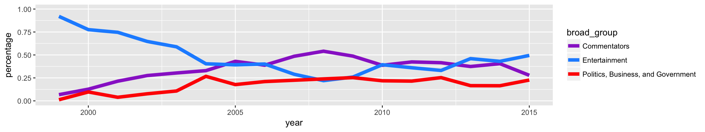

4.3 Data Wranging: Joining Data Frames

Additional reading:

Wickham and Grolemund on relational data
Chapter 10 of Data Computing by Kaplan

In this section you will need the following packages:

library(tidyverse)
library(ggplot2)
library(ggmap)
library(lubridate)

A join is a data verb that combines two tables.

These are called the left and the right tables.

There are several kinds of join.

All involve establishing a correspondance — a match — between each case in the left table and zero or more cases in the right table.
The various joins differ in how they handle multiple matches or missing matches.

Establishing a match between cases

A match between a case in the left table and a case in the right table is made based on the values in pairs of corresponding variables.

You specify which pairs to use.
A pair is a variable from the left table and a variable from the right table.
Cases must have exactly equal values in the left variable and right variable for a match to be made.

As an example, we’ll examine the following two tables on grades and courses. The Grades file has one case for each class of each student, and includes variables describing the ID of the student (sid), the ID of the session (section), and the grade received. The Courses table has variables for the ID of the session (section), the department (coded), the level, the semester, the enrollment, and the ID of the instructor (iid). We show a few random rows of each table below.

Grades <- read_csv("http://tiny.cc/mosaic/grades.csv")
Grades <- Grades %>%
  select(sid,sessionID,grade) %>%
  distinct(sid,sessionID,.keep_all = TRUE)

Table 4.9: Student grades.
sid	sessionID	grade
S31680	session3521	A-
S31242	session2933	C+
S32127	session2046	B
S32058	session2521	B+

Courses <- read_csv("http://tiny.cc/mosaic/courses.csv")

Table 4.10: Information about each course section.
sessionID	dept	level	sem	enroll	iid
session2568	J	100	FA2002	15	inst223
session1940	d	100	FA2000	16	inst409
session3242	m	200	SP2004	30	inst476
session3132	M	100	SP2004	18	inst257

Mutating joins

The first class of joins are mutating joins, which add new variables (columns) to the left data table from matching observations in the right table.⁸

The main difference in the three mutating join options in this class is how they answer the following questions:

What happens when a case in the right table has no matches in the left table?
What happens when a case in the left table has no matches in the right table?

Three mutating join functions:

left_join(): the output has all cases from the left, regardless if there is a match in the right, but discards any cases in the right that do not have a match in the left.
inner_join(): the output has only the cases from the left with a match in the right.
full_join(): the output has all cases from the left and the right. This is less common than the first two join operators.

When there are multiple matches in the right table for a particular case in the left table, all three of these mutating join operators produce a separate case in the new table for each of the matches from the right.

One of the most common and useful mutating joins in one that translates levels of a variable to a new scale. For example, below we’ll see a join that translates letter grades (e.g., “B”) into grade points (e.g., 3).

Exercise 1. Your First Join: Determine the average class size from the viewpoint of a student and the viewpoint of the Provost / Admissions Office.

Answer:

The Provost counts each section as one class and takes the average of all classes. We have to be a little careful and cannot simply do mean(Courses$enroll), because some sessionIDs appear twice on the course list. Why is that?⁹ We can still do this from the data we have in the Courses table, but we should aggregate by sessionID first:

CourseSizes<-Courses %>%
  group_by(sessionID) %>% 
  summarise(total_enroll=sum(enroll))
mean(CourseSizes$total_enroll)
## [1] 21.45251

To get the average class size from the student perspective, we can join the enrollment of the section onto each instance of a student section. Here, the left table is Grades, the right table is CourseSizes, we are going to match based on sessionID, and we want to add the variable total_enroll. We’ll use a left_join since we aren’t interested in any sections from the CourseSizes table that do not show up in the Grades table; their enrollments should be 0, and they are not actually seen by any students. Note, e.g., if there were 100 extra sections of zero enrollments on the Courses table, this would change the average from the Provost’s perspective, but not at all from the students’ perspective.

Note: If the by= is omitteed from a join, then R will perform a natural join, which matches the two table by all variables they have in common. In this case, the only variable in common is the sessionID, so we would get the same results by omitting the second argument. In general, this is not reliable unless we check ahead of time which variables the tables have in common. If two variables to match have different names in the two tables, we can write by=c("name1"="name2").

EnrollmentsWithClassSize <- Grades %>% 
  left_join(CourseSizes, by=c("sessionID"="sessionID")) %>%
  select(sid,sessionID,total_enroll)

Table 4.11: Student enrollments with the section size.
sid	sessionID	total_enroll
S31680	session3521	12
S31242	session2933	18
S32127	session2046	34
S32058	session2521	15

AveClassEachStudent<-EnrollmentsWithClassSize %>%
  group_by(sid) %>%
  summarise(ave_enroll = mean(total_enroll, na.rm=TRUE))

Table 4.12: Average class size seen by each individual student.
sid	ave_enroll
S31677	23.83333
S31242	26.72727
S32121	23.33333
S32052	23.63636

The na.rm=TRUE here says that if the class size is not available for a given class, we do not count that class towards the student’s average class size. What is another way to capture the same objective? We could have used an inner_join instead of a left_join when we joined the tables to eliminate any entries from the left table that did not have a match in the right table.

Now we can take the average of the AveClassEachStudent table, counting each student once, to find the average class size from the student perspective:

mean(AveClassEachStudent$ave_enroll)
## [1] 24.41885

We see that the average size from the student perspective (24.4) is greater than the average size from the Provost’s perspective (21.5). It is a fun probability exercise to prove that this fact is always true!!

Filtering joins

The second class of joins are filtering joins, which select specific cases from the left table based on whether they match an observation in the right table.

semi_join(): discards any cases in the left table that do not have a match in the right table. If there are multiple matches of right cases to a left case, it keeps just one copy of the left case.
anti_join(): discards any cases in the left table that have a match in the right table.

A particularly common employment of these joins is to use a filtered summary as a comparison to select a subset of the original cases, as follows.

Example 4.1 (semi_join to compare to a filtered summary) Find a subset of the Grades data that only contains data on the four largest sections in the Courses data set.

Solution.

LargeSections<-Courses %>%
  group_by(sessionID) %>%
  summarise(total_enroll=sum(enroll)) %>%
  top_n(total_enroll, n=4)
GradesFromLargeSections <- Grades %>%
  semi_join(LargeSections)

Exercise 2. Semi Join: Use semi_join() to create a table with a subset of the rows of Grades corresponding to all classes taken in department J.

Answer:

There are multiple ways to do this. We could do a left join to the Grades table to add on the dept variable, and then filter by department, then select all variables except the additional dept variable we just added. Here is a more direct way with semi_join that does not involve adding and subtracting the extra variable:

JCourses <- Courses %>%
  filter(dept=="J")
JGrades <- Grades %>% 
  semi_join(JCourses)

Let’s double check this worked. Here are the first few entries of our new table:

Table 4.13: Student enrollments in Department J.
sid	sessionID	grade
S31185	session1791	A-
S31185	session1792	B+
S31185	session1794	B-
S31185	session1795	C+

The first entry is for session1791. Which department is that?

(Courses%>%filter(sessionID=="session1791"))
## # A tibble: 1 x 6
##     sessionID  dept level    sem enroll     iid
##         <chr> <chr> <int>  <chr>  <int>   <chr>
## 1 session1791     J   100 FA1993     22 inst223

But that only checked the first one. What if we want to double check all of the courses included in Table 4.13? We can add on the department and do a group by to count the number from each department in our table.

JGrades %>%
  left_join(Courses) %>%
  group_by(dept) %>%
  summarise(total=n())
## # A tibble: 1 x 2
##    dept total
##   <chr> <int>
## 1     J   148

More join practice

For each of these questions, say what tables you need to join and identify the corresponding variables.

How many student enrollments in each department?
What’s the grade-point average (GPA) for each student?
What fraction of grades are below B+?
What’s the grade-point average for each department or instructor?

Bicycle-Use Patterns

In this activity, you’ll examine some factors that may influence the use of bicycles in a bike-renting program. The data come from Washington, DC and cover the last quarter of 2014.

Two data tables are available:

Trips contains records of individual rentals
Stations gives the locations of the bike rental stations

Figure 4.2: A typical Capital Bikeshare station. This one is at Florida and California, next to Pleasant Pops.

Figure 4.3: One of the vans used to redistribute bicycles to different stations.

Here is the code to read in the data:¹⁰

data_site <- 
  "https://tiny.cc/dcf/2014-Q4-Trips-History-Data-Small.rds" 
Trips <- readRDS(gzcon(url(data_site)))
Stations<-read_csv("https://tiny.cc./dcf/DC-Stations.csv")

The Trips data table is a random subset of 10,000 trips from the full quarterly data. Start with this small data table to develop your analysis commands. When you have this working well, you can access the full data set of more than 600,000 events by removing -Small from the name of the data_site.

Exercise 3. Warm-Up: Temporal patterns

It’s natural to expect that bikes are rented more at some times of day, some days of the week, sme months of the year than others. The variable sdate gives the time (including the date) that the rental started.

Make the following plots and interpret them:

A density plot of the events versus sdate. Use ggplot() and geom_density().
A density plot of the events versus time of day. You can use mutate with lubridate::hour(), and lubridate::minute() to extract the hour of the day and minute within the hour from sdate. Hint: A minute is 1/60 of an hour, so create a field where 3:30 is 3.5 and 3:45 is 3.75.
A histogram of the events versus day of the week.
Facet your graph from (b) by day of the week. Is there a pattern?

The variable client describes whether the renter is a regular user (level Registered) or has not joined the bike-rental organization (Causal). Do you think these two different categories of users show different rental behavior? How might it interact with the patterns you found in Exercise 3?

Exercise 4. Customer Segmentation Repeat the graphic from Exercise 3 (d) with the following changes:

Set the fill aesthetic for geom_density() to the client variable. You may also want to set the alpha for transparency and color=NA to suppress the outline of the density function.
Now add the argument position = position_stack() to geom_density(). In your opinion, is this better or worse in terms of telling a story? What are the advantages/disadvantages of each?
Rather than faceting on day of the week, create a new faceting variable like this: mutate(wday = ifelse(lubridate::wday(sdate) %in% c(1,7), "weekend", "weekday")). What does the variable wday represent? Try to understand the code.
Is it better to facet on wday and fill with client, or vice versa?
Of all of the graphics you created so far, which is most effective at telling an interesting story?

Exercise 5. Mutating join practice: Spatial patterns

Use the latitude and longitude variables in Stations to make a visualization of the total number of departures from each station in the Trips data. To layer your data on top of a Google map, start your plotting code as follows:

myMap <- get_map(location="Logan Circle",source="google",maptype="roadmap",zoom=13)
ggmap(myMap) + ...

Only 14.4% of the trips in our data are carried out by casual users.¹¹ Create a map that shows which area(s) of the city have stations with a much higher percentage of departures by casual users. Interpret your map.

Exercise 6. Filtering join practice: Spatiotemporal patterns

Hint for part(a): as_date(sdate) converts sdate from date-time format to date format.

Make a table with the ten station-date combinations (e.g., 14th & V St., 2014-10-14) with the highest number of departures, sorted from most departures to fewest.
Use a join operation to make a table with only those trips whose departures match those top ten station-date combinations from part (a).
Group the trips you filtered out in part (b) by client type and wday (weekend/weekday), and count the total number of trips in each of the four groups. Interpret your results.

The fivethirtyeight package has more recent data.↩
The label=TRUE argument tells month to return a string abbreviation for the month instead of the month’s number.↩
The point of the lubridate::dmy() function is to convert the character-string date stored in the CSV to a POSIX date-number.↩
Hints for part (c) of Exercise ??: You’ll have to make up a y-coordinate for each label. You can set the orientation of each label with the angle aesthetic.↩
Note that when multiple people appeared together, each person receives their own line.↩
Hint: the function rowSums() adds up all of the entries in each row of a table. Try using it in a mutate.↩
Hint: gather uses the dplyr::select() notation, so you can, e.g., list the columns you want to select, use colon notation, or use contains(a string). See Wickham and Grolemund for more information.↩
There is also a right_join() that adds variables in the reverse direction from the left table to the right table, but we do not really need it as we can always switch the roles of the two tables.↩
They are courses that are cross-listed in multiple departments!↩
Important: To avoid repeatedly re-reading the files, start the data import chunk with {r cache = TRUE} rather than the usual {r}.↩
We can compute this statistic via mean(Trips$client=="Casual").↩